Algorithms for Causal Discovery

February 7, 2017

This article considers the problem of estimating the structure of the causal DAG given some observational data.

How difficult is it to learn a DAG?

The number of DAGs for $n$ nodes increases super exponentially in $n$.

The entire list upto $n=40$ can be found here.

From what I have read so far, there are three major methods to learn causal structures. They are

1. Methods based on Independence Tests
2. Score based methods
3. Methods based on making assumptions about the distribution

The first two methods estimate the true causal DAG upto the Markov equivalent class. What that means is that the final DAG that is output from the algorithm may contain undirected edges (formally called CPDAG - completed partially directed acyclic graph). Algorithms in the third method claim to estimate the true causal DAG, assuming that the required conditions are met.

The following is an overview of the algorithms in each method.

Methods based on Independence Tests

Consider three variables $A$, $B$ and $C$. Let us assume that there are no unobserved variables. These variables can be arranged in four ways.

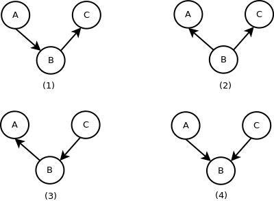
Figures 1,2 and 3 represent the same set of conditional independence relationships between the three variables, and Figure 4 represents a different set of conditional independence relationships.

Let us consider Figure 4, with $A$ and $C$ both pointing towards $B$ (This is sometimes called a collider). $A$ and $C$ are dependent conditioned on $B$. One way to understand this is to consider $A$ and $C$ as the outcomes of coin tosses of two separate coins, and $C$ as a random variable that takes the value of $1$ if both coins give the same outcome, and $0$ otherwise. The two coin tosses are independent unconditionally. But, once we know the value of $B$, $A$ and $C$ are dependent on each other.

Algorithms based on Independence Tests primarily use this property of colliders to identify $v$ structures from the data. However, they cannot orient all edges because conditional independence testing cannot distinguish between Figures (1), (2) and (3). Hence, these algorithms can estimate the causal DAG upto the Markov equivalence class.

Score Based Methods

In score based methods, we assign a score to every DAG depending on the goodness of fit with the data, and search over the space of DAGs to find the one with the best score. The number of DAGs for $n$ variables grows super-exponentially, as seen earlier.

Greedy search algorithms are used to find the best scoring DAG.

Other Methods

If we consider the framework of Structural Equation Models (also Structural Causal Models), making some assumptions about the model helps us recover the true DAG.

Let us formally define Structural Equation Models (SEM). For some set of random variables $X={X_1,..,X_p}$, the general SEM is defined as a set of functions \(X_i = f_i(PA_i, N_i)\) where $N_1,..,N_p$ are mutually independent. $PA_i$ denotes the parents of $X_i$ in the DAG, $N_i$ is the noise variable and $f_i$ is a function from $\mathbb{R}^{|PA_i|+1} \rightarrow \mathbb{R}$. Depending on the kind of assumption made on $f_i$, there are three different approaches that I have come across.

Linear Gaussian Acyclic Model (LinGAM)

Consider a linear SEM \(X_j = \sum\limits_{k \in PA_j} \beta_{jk} X_k + N_j\) where all $N_j$ are mutually independent and are non-Gaussian, and $\beta_{jk} \ne 0$ for all $k \in PA_j$. This SEM is also called as LinGAM.

Basically, this model makes the assumption that every variable in the SEM depends linearly on its parents. In 2006, it was proved that the original DAG is identifiable from this SEM. A practical method for finite data uses Independent Component Analysis (ICA) to estimate the true DAG. The original paper can be found here

Causal Additive Models (CAM)

Consider an SEM of the form \(X_j = \sum \limits_{k \in PA_j} f_{j,k}(X_k) + N_j\) with $N_1, …, N_p$ mutually independent with $N_j=\mathcal{N}(0, \sigma_j^2)$, $\sigma_j^2 > 0$ for all $j$. Also, all $f_{j,k}(.)$ are smooth functions from $\mathbb{R} \rightarrow \mathbb{R}$.

In other words, we assume that each variable is determined by a sum of functions of its parents with a Gaussian noise component. It has been proved that if the functions $f_{j,k}$ are non-linear, the DAG is identifiable from the joint distribution. This paper provides a broad framework to identify the DAG from finite data, assuming the distribution meets the conditions mentioned earlier. This method is feasible for upto 200 variables.

Additive Noise Models (ANM)

Consider the Additive Noise Model (ANM) which is of the form \(X_j = f_j(PA_j) + N_j\) where $PA_j$ denotes the parents of $X_J$, functions $f_j$ are non-constant and all noise variables $N_j$ are mutually independent. If we additionally assume that the noise variables have non-vanishing densities and the functions $f_j$ are three times continuously differentiable, it has been proved that the original DAG is identifiable from the joint distribution. One practical method for finite data is Regression with Subsequent Independence Test (RESIT). More about the method can be found here. ANM is more general than CAM. This method is feasible for upto 20 variables.