Estimating Parameters in a Bayesian Network
September 23, 2016
In this article, I will describe how to find the maximum likelihood estimates for parameters of a Bayesian Network. Intutively, a Bayesian Network provides a way to capture dependecies between different variables that we are interested in.
Consider some dataset $D$ which contains a set of variables $V=\{V_1,..,V_n\}$. Here, we assume that the variables are categorical - basically, it means that the set of possible values that the variable can take is finite. The joint probability distribution describes the way the values of the dataset is spread out. Storing the joint probability distribution explicitely is costly, but Bayesian Networks provide an efficient alternative.
In a Bayesian Network, the joint distribution can be factored into a set of terms as follows
\[Pr(V) = \prod_{i=1}^nPr(V_i\mid \pi_i)\]where $\pi_i$ is a subset of $V$ called the parents of $V_i$. If we draw a graph such that there is an edge to $V_i$ from all variables in $\pi_i$, we obtain the graph assciated with the Bayesian Network. We make the additional assumption that this graph is a DAG.
Let us take an example. Consider the DAG below.

The joint probability distribution can be factored as follows \(Pr(A,B,C,D,E,F)=Pr(A).Pr(B).Pr(C \mid A,B).Pr(D \mid C).Pr(E \mid C).Pr(F \mid E)\)
An important independence assumption in Bayesian Networks is that every node in the DAG is independent of its non-descendants, given its parents. In the previous example, given $C$, $E$ is independent of $A$ and $B$.
This article mainly deals with the estimation of parameters for the Bayesian Network, so it assumes that the structure of the network (ie, the DAG between different nodes) is already known. Since we know that the joint probability distribution can already be factored into a set of conditional probability distributions, if we can somehow estimate these conditional distributions, then we are done.
The method to find the maximum likelihood estimate for the parameters of the network is so simple, that it almost seems trivial. Consider the DAG given above. Suppose we want to find the conditional distribution $Pr(C \mid A,B)$. $C$ takes a value from ${x,y}$, $A$ takes a value from ${1,2}$ and $B$ is always $3$. We will need to construct the following table from our dataset -
| C | A | B | # of rows in $D$ |
|---|---|---|---|
| x | 1 | 3 | - |
| x | 2 | 3 | - |
| y | 1 | 3 | - |
| y | 2 | 3 | - |
For every value that $C$ takes and for every possible combination of values for $\pi_i$ (the parents of $C$), we need to find how many times this combination occurs in the dataset. Basically, for every possible combination of values for $V_i$ and $\pi_i$ we want to count the number of rows in the dataset that contain this combination. More formally, the maximum likelihood estimate is given by
\[\theta_{ijk} = \frac {n_{ijk}} {n_{ij}}\]where ${n_{ijk}}$ is the number of times that variable $i$ takes the value $j$ with its parents having the $k^{th}$ configuration, and $n_{ij}$ is the number of times that variable $i$ takes the value $j$ in the dataset.
If you notice, we haven’t included $n_{ij}$ in the table that we created. This is because $n_{ijk}$ constitutes the sufficient statistics for the distribution (or, the distribution is completely described by the quantity $n_{ijk}$).
Expedia Hotel Recommendations Competetion on Kaggle
In 2016, Kaggle hosted the Expedia Hotel Recommendations competetion. Participants were required to contextualize customer data and predict the likelihood that a user would stay at 100 different hotel groups. Putting aside the data leak, the “counting solution” was quite popular in the discussion forums. While the solution evidently “worked” and gave reasonable results, no one seemed to be able to give a theoretical basis to what the underlying model and assumptions might have been.
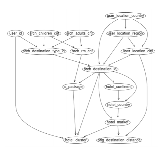
Here is one possible explanation as to why the solution worked. We constructed the following Bayesian Network based on our knowledge and understanding.

For every record in the test file, we are given the values for all nodes except hotel_cluster. We used quantile binning to discretize continuous variables. The competetion requires that we output the top 5 most likely hotel_cluster values. So, all we did was calculate the maximum likelihood estimate for all possible hotel_cluster values and picked the top 5.